 I am working at the
 Towards a Synthetic Benchmark to Assess VM Startup, Warmup, and Cold-Code Performance
One of the hard problems in language implementation research is benchmarking. Some people argue, we should benchmark only applications that actually matter to people. Though, this has various issues. Often, such applications are embedded in larger systems, and it’s hard to isolate the relevant parts. In many cases, these applications can also not be made available to other researchers. And, of course, things change over time, which means maintaining projects like DaCapo, Renaissance, or Jet Stream is a huge effort.
Which brought me to the perhaps futile question of how we could have more realistic synthetic benchmarks. ACDC and ACDC-JS are synthetic garbage collection benchmarks. While they don’t seem to be widely used, they seemed to have been a useful tool for specific tasks. Based on observing metrics for a range of relevant programs, these synthetic benchmarks were constructed to be configurable and allow us to measure a range of realistic behaviors.
I am currently interested in the startup, warmup, and cold-code performance of virtual machines, and want to study their performance issues. To me it seems that I need to look at large programs to get interesting and relevant results. With large, I mean millions of lines of code, because that’s where our systems currently struggle. So, how could we go about to create a synthetic benchmark for huge code bases?
Generating Random Code that Looks Real
In my last two blog posts [1, 2], I looked at the shape of large code bases in Pharo and Ruby to obtain data for a new kind of synthetic benchmark. I want to try to generate random code that looks “real”. And by looking real I mean for the moment that it is shaped in a way that is similar to real code. This means, methods have realistic length, number of local variables, and arguments. For classes, they should have a realistic number of methods and instance variables. In the last two blog posts, I looked at the corresponding static code metrics to get an idea of how large code bases actually look like.
In this post, I am setting out to use the data to get a random number generator that can be used to generate “realistic looking” code bases. Of course, this doesn’t mean that the code does do anything realistic.
Small steps… One at a time… 👨🏼🔬
So, let’s get started by looking at how the length of methods looks like in large code bases.
Before we get started, just one more simplification: I will only consider methods that have 1 to 30 lines (of code). Setting an upper bound will make some of the steps here simpler, and plots more legible.
And a perhaps little silly, but nonetheless an issue, it will avoid me having to change one of the language implementations I am interested in, which is unfortunately limited to 128 bytecodes and 128 literals (constants, method names, etc.), which in practice translates to something like 30 lines of code. While this could be fixed, let’s assume 30 lines of code per method ought to be enough for anybody…
Length of Methods
When it comes to measuring the length of methods, there are plenty of possibly ways to go about. Pharo counts the non-empty lines. And for Ruby, I counted either all lines, or the lines that are not just empty and not just comments.
The histogram below shows the results for methods with 1-30 lines.
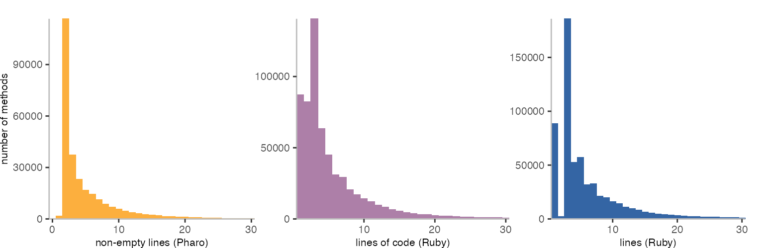
Despite difference in languages and metrics, we see a pretty similar shape. Perhaps with the exception of the methods with 1-3 lines.
Generating Realistic Method Length from Uniform Random Numbers
Before actually generating method length randomly, let’s define the goal a bit more clearly.
In the end, I do want to be able to generate a code base where the length of methods has a distribution very similar to what we see for Ruby and Pharo.
Though, the random number generators we have in most systems generate numbers in a uniform distribution typically in the range from 0 to 1. This means, each number between 0 and 1 is going to be equally likely to be picked. To get other kinds of distributions, for instance the normal distribution, we can use what is called the inverted cumulative distribution function. When we throw our uniformly distributed numbers into this function, we should end up with random numbers that are distributed according to the distribution that we want.
One of the options to do this would be:
- determine the cumulative distribution of the method length
- approximate a function to represent the cumulative distribution
- and invert the function
I found this post here helpful. Though, I struggled defining a good enough function to get results I liked.
So, instead, let’s do it the pedestrian way:
- calculate the cumulative sum for the method length (cumulative distribution)
- normalize it to the sum of all lengths
- use the result to look up the desired method length for a uniform random number
Determining the Cumulative Distribution
Ok, so, the first step is to determine the cumulative distribution. Since we have the three different cases for Pharo, Ruby with all lines and lines of code, this is slightly more interesting.

The plot above shows the percentage of methods that have a length smaller or equal to a specific size.
So, the next question is, which metrics should I choose? Since the data is a bit noisy, especially for small methods, let’s try and see what the different types of means give us.
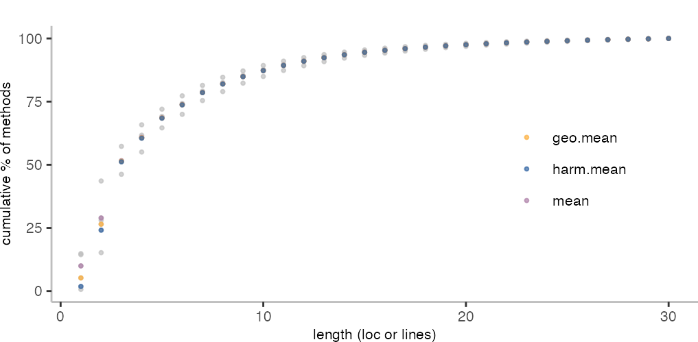
From the above plot, the geometric mean seems a good option. Mostly because I don’t want to have a too high and too low number of methods with a single line.
Using the geometric mean, gives us the following partial cumulative distribution table:
| length | cum.perc |
|---|---|
| 1 | 0.0520631 |
| 2 | 0.2647386 |
| 3 | 0.5137505 |
| 4 | 0.6068893 |
| 5 | 0.6851248 |
| 6 | 0.7377313 |
| 7 | 0.7861208 |
| 8 | 0.8200427 |
| 9 | 0.8490800 |
In R, the language I use for these blog posts,
I can then use something like the following to take a uniform random number
from the range of 0-1 to determine the desired method length in the range
of 1-30 lines (u being here the random number):
loc_from_u <- function (u) {
  Position(function (e) { u < e }, cumulative_distribution_tbl)
}
There are probably more efficient ways of going about it. I suppose a binary search would be a good option, too.
The general idea is that with our random number u,
we find the last position in our array with the cumulative distribution,
where u is smaller than the value in the array at that position.
The position then corresponds to the desired length of a method.
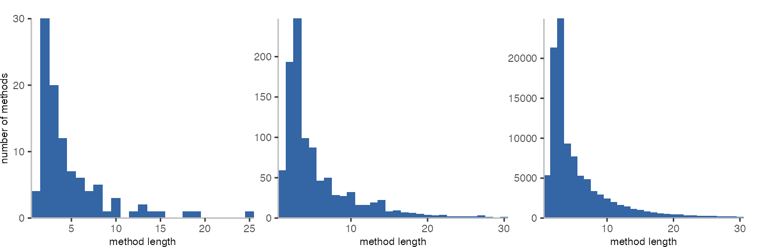
As a test, the three plots above are generated from 100, 1,000, and 100,000 uniformly distributed random numbers, and it looks pretty good. Comparing to the very first set of plots in this post, this seems like a workable and relatively straightforward approach.
To use these results and generate methods of realistic sizes in other languages, the full cumulative distribution is as follows: [0.0520631241473676, 0.264738601144803, 0.51375051909561, 0.606889305644881, 0.685124787391578, 0.737731315373305, 0.786120782303596, 0.820042695503066, 0.849080035429476, 0.872949669419948, 0.893437469528804, 0.909716501217452, 0.923766913966731, 0.935357118689879, 0.945074445934092, 0.953001059092301, 0.959743413722937, 0.965457396618992, 0.97072530951053, 0.975142363341172, 0.979105371695575, 0.982654867280203, 0.985723232507825, 0.988399223471247, 0.990960559703172, 0.993172997617124, 0.9951015059492, 0.996855138214434, 0.998541672752458, 1].
Method Arguments and Local Variables
With the basics down, we can look at the number of arguments and local variables of methods. One thing I haven’t really thought about in the previous posts is that there’s a connection between the various metrics. They are not independent of each other.
Perhaps this is most intuitive for the number of local variables a method has. We wouldn’t expect a method with a single line of code to have many local variables, while longer methods may tent to have more local variables, too.
Number of Method Arguments
Let’s start out by looking at how method length and number of arguments relate to each other.
I’ll use the cumulative distribution for these plots, since that’s what I am looking for in the end.
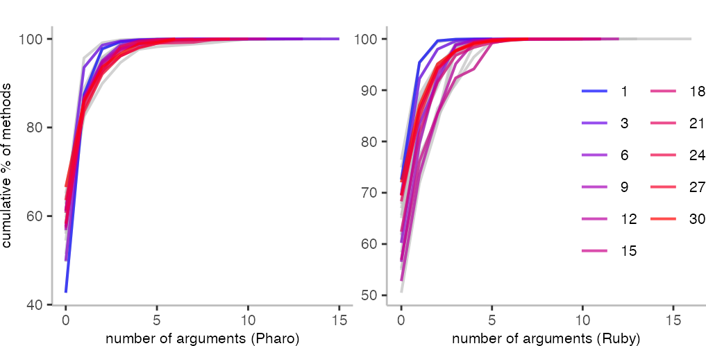
The two plots above show for each method length from 1-30 a line (so, this is where limiting the method length becomes actually handy). Though, because there are many, I highlight only every third length, including length 1 methods. The bluest blue is length 1, and the red is length 30.
We can see here differences between the languages. For instance, for methods with only 1 line in Pharo, only ≈45% of them have no argument. While for Ruby methods, that’s perhaps around 70%.
The other interesting bit that is clearly visible is that the number of arguments doesn’t have a simple direct relationship to length. Indeed, longer methods seem to have more likely fewer arguments. While medium length methods are more likely to have a few more arguments, at least for the Ruby data this seems to be the case.
So, from these plots, I conclude that I actually need a different cumulative distribution table for each method length. Since we saw how they look for method length, I won’t include the details. Though, of course happy to share the data if anyone wants it.
Number of Methods Locals
Next up, let’s look at the number of locals.
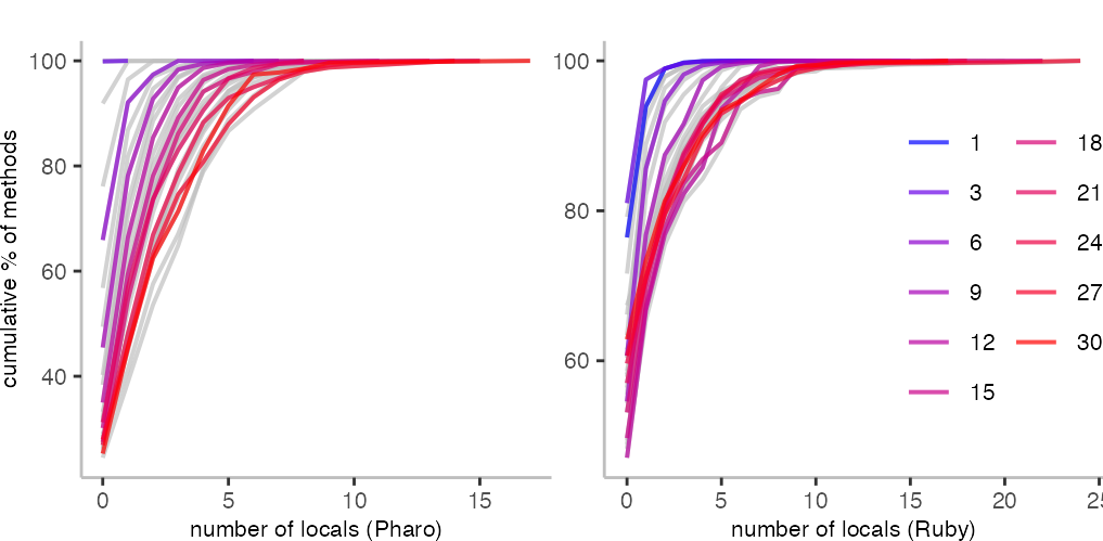
For the Pharo data, it’s not super readable, but basically 100% of methods of length 1 have zero local variables. Compared to the plot on arguments, we also see a pretty direct relationship to length, because the blue-to-red gradient comes out nicely in the plot.
In the case of Ruby, this seems to be similar, but perhaps not as cleanly as for Pharo. The different y-axis start points are also interesting, because they indicate that longer methods in Pharo are more likely to have arguments than in Ruby.
For generating code, I suppose one needs to select the distributions that are most relevant for one’s goal.
Classes: Number of Methods and Fields
After looking at properties for methods, let’s look at classes. I fear, these various metrics are pretty tangled up, and one could probably find many more interesting relationships between them, but I’ll restrict myself for this post to the most basic ones. First I’ll look at the cumulative distribution for the number of methods per class, and then look at the number of instance variables classes have depending on their size.
Number of Methods per Class
I’ll restrict my analysis here to classes with a maximum of 100 methods, because the data I have does not include enough classes with more than 100 methods.
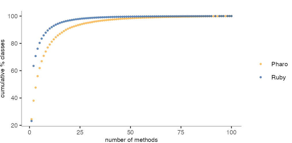
As we saw in the previous post, we can here see that Ruby has many more classes with only one or two methods. On the other hand, it seems to have slightly fewer larger classes. Expressed differently, about 60% of all Ruby methods (which includes closures) have 1 or 2 arguments, while in the case of Pharo (where closures where ignored), we need about 5-6 arguments to reach the same level.
Number of Fields for Classes with a Specific Number of Methods
For the number of fields of a class, I can easily look at the relation to the number of methods, too.
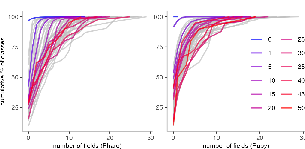
In the two plots above, we see that there is an almost clear relationship between the number of methods and fields. A class having more methods seems to indicate that is may have more fields. For both languages, there’s some middle ground where things are not as clear, but at least for classes with fewer methods, it seems to hold well.
Conclusion
The most important insight for me from this exercise is that I can generate code that has a realistic shape relatively straightforwardly based on the data collected.
At least, it seems easy and reliable to get a random number distribution of the desired shape.
In addition, we saw that there are indeed interdependencies between the different metrics. This is not too surprising, but something one needs to keep in mind when generating “realistic” code.
So, where from here? Well, I already got a code generator that can generate millions of lines of code that use basic arithmetic operations. The next step would be to fit this code into a shape that’s more realistic. One problem I had before is that my generated code started stressing things like the method look up, in a way real code doesn’t. Shaping things more realistically, will help avoid optimizing things that may not matter. Then again, we see pathologic cases also in real code.
Ending this post, there are of course more open questions, for instance:
- how do I generate realistic behavior?
- do large chunks of generated code allow me to study warmup and cold-code performance in a meaningful way? Or asked differently, does the generated code behave similar enough to real code?
- which other metrics are relevant to generate realistic code?
Though, I fear, I’ll need to wait until spring or summer to revisit those questions.
For suggestions, comments, or questions, find me on Twitter @smarr.